Coding A Neural Network In Matlab

Published on: February 21, 2018April 18, 2018Author: Mihai ErmaliucComment: 0

This post will guide you through the process of building your own feed-forward multilayer neural network in Matlab in a (hopefully) simple and clean style. It is designed for people who already have some coding experience as well as a basic understanding of what neural networks are and want to get a bit deeper into the way they work. You will also need basic knowledge of linear algebra (matrix multiplication) and derivatives in order to understand the process in depth. The next post will explain and implement the backpropagation training algorithm in the same way. Following posts will get a bit deeper into details such as choosing the activation functions, network architecture, weights initialization etc.

The network will have a configurable number of layers, activation functions on each layer as well as cost functions.

The following sections will briefly explain both the concept and the implementation. The source code for the network together with training and examples is available here. You can run Test2dReg.m for a demo.

The basic structure of a feed-forward neural network

This article will review but does not necessarily aim to give you the basic understanding of neural networks. There are numerous resources on the internet that cover this topic, some of them here:

https://en.wikipedia.org/wiki/Feedforward_neural_network
https://hackernoon.com/everything-you-need-to-know-about-neural-networks-8988c3ee4491
Although not directed to neural networks only, I would also recommend Andrew Ng’s excellent introductory Machine Learning course here. Hint: if you understand logistic regression then you understand what a neuron is.

A neural network is a collection of neurons structured in successive layers. A neuron is a unit that owns a vector of values W (called weights), takes another vector of values X as input and calculates a single output value y based on it:

$y = a( s(X) )$

where s(X) is a function performing a weighted summation of the elements of the input vector. It is usual to add a so-called bias to the input of each neuron (see here a good explanation). This is a term that does not depend on the input vector X but only on the corresponding weight value and is modeled in the following equation by adding an artificial input fixed to 1:

$\inline X = (x_0=1, x_1,x_2,...,x_n)$

$s(X) = \sum_{i=0}^{n}w_ix_i$

The function a(x) is called the activation function and performs a non-linear transform of the summation result. The activations allow the network to learn complex non-linear functions. There are many such functions, but some widely used are the logistic, hyperbolic tangent(tanh) and linear rectifier (RELU). While the logistic function has been used widely in the past, the hyperbolic tangent makes the learning process easier (LeCun et al, 1998). The linear rectifier is preferred for deep networks, being computationally cheaper and not prone to vanishing gradients during training (more on this in the next post).

Logistic	Hyperbolic tangent (tanh)	Linear rectifier RELU
$a(x) = \frac{1}{1+e^{-x}}$	$a(x) = \frac{e^x - e^{-x}}{e^x + e^{-x}}$	$a(x) = min(0, x)$

These neurons are grouped in successive layers (L₁, L₂, …, L_K) with L₁ being the input layer, L_K the output layer and the rest of them generically called hidden layers. Each neuron on layer k is “connected” to all the neurons on layer k-1. This connection means that the neuron owns a vector of weights with the same size as the number of neurons on layer k-1 and during operation will receive as input the output values of these neurons. The bias unit can be modeled by adding a fake neuron on each layer with it’s output always equal to 1. The neurons on the input layer are not connected to anything (there is no back layer) and nothing connects to the neurons on the output layer. Also the bias units (b in the image below) are optional, not connected to the previous layer and not present on the output layer.

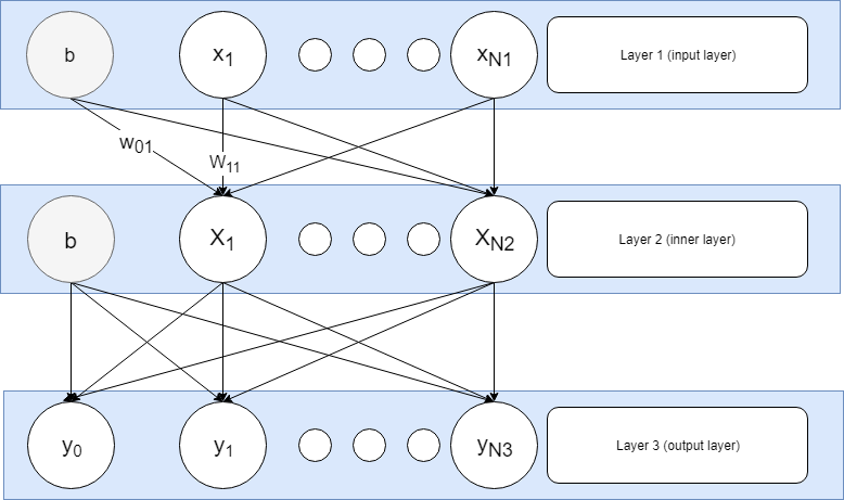
Fig. 1. Neural network with 3 layers and unspecified number of neurons

Neurons on a layer act simultaneously while the layers act in succession. During operation a vector of input values is fed into the input layer. The neurons on the next layer will take the input values and calculate their own outputs as described above, then the next layer will act similarly up to the output layer, whose neurons’ values are effectively the output of the network.

The vectorized formulas

The transfer of values from one layer to another can be expressed using matrix operations, which is very convenient since they can be performed efficiently in many environments (i.e. Python’s numpy library, Matlab, Octave etc.). It is easy to see that if we collect all the weights connecting layer k to k-1 into a matrix where column n stores the weights from each neuron on layer k-1 to neuron n on layer k:

$W^{(k)} = \begin{pmatrix} w_{01}\ \ \ w_{02}\ \ \ ... \ \ \ w_{0N_k} \\ w_{11} \ \ \ w_{12} \ \ \ ... \ \ \ w_{1N_k} \\ .................... \\ w_{N_{k-1}1 } \ w_{N_{k-1}2} \ w_{N_{k-1}N_k } & \end{pmatrix}$ , where N_k is the number of neurons on layer k excluding the bias unit.

Then calculating the output of layer k can be expressed using matrix multiplication for the summation:

$S^{(k)} = X^{(k-1)} W^{(k)} = (x_0, x_1, ..., x_N_{k-1})\begin{pmatrix} w_{01}\ \ \ w_{02}\ \ \ ... \ \ \ w_{0N_k} \\ w_{11} \ \ \ w_{12} \ \ \ ... \ \ \ w_{1N_k} \\ .................... \\ w_{N_{k-1}1 } \ w_{N_{k-1}2} \ w_{N_{k-1}N_k } & \end{pmatrix} = (\sum_{i=0}^{N_{k-1}}w_{i1}x_i,\sum_{i=0}^{N_{k-1}}w_{i2}x_i, ..., \sum_{i=0}^{N_{k-1}}w_{iN_k}x_i)= (s_1, s_2, ..., s_N_k)$

Note that in the above formula rows start from 0 while columns from 1. This is because neuron 0 (the bias unit) on layer k does not connect to the back layer since it will always output 1 (hence the absence of column 0), while the rest of the neurons on layer k connect to the bias unit on layer k-1 (hence the presence of line 0).

And finally applying the activation a on each element of the S vector and adding the output of the bias unit:

$X^{(k)} = a^{(k)}(S^{(k)}) = (1, a^{(k)}(s_1), a^{(k)}(s_2), ..., a^{(k)}(s_N_k))$

Note that this is not quite the standard form, you might usually find the formula with the weights matrix transposed and the bias separated. This is however how it will be implemented in code.

Modeling the network – the NeuralNetwork class

The choice of design is not the best nor intended to achieve high performance but rather to keep the code clean and clear. Also it is not intended as fully object-oriented but takes advantage of Matlab’s classes to group multiple functions in a single file.

The previous section gives a clearer picture of the data structures we need in order to implement such a network: weights, neuron layers, activation functions per layer. To prepare for the next post showing how networks are trained we will add 3 more elements: the derivative of each activation function, a cost function and also its derivative.

The code will be structured in a single class, NeuralNetwork, storing all the necessary properties: . It will also have methods to build and operate the network.

Let’s start with the empty class which we will fill in the following sections.

classdef NeuralNetwork<handle

    properties
        ...
    end
    
    methods       
        function network = NeuralNetwork(nInputs, biasPresent)
        end
        
        function addLayer(network, nNeuronsInLayer, biasPresent, activationFn, activationFnDv)
            ...
        end
        
        function output = calculateOutput(network, X)
            ...
        end
              
        function initWeights(network, layers, range)
            ...
        end               
       
    end
end

All the properties except for the cost function are per network layer, hence will be stored in ordered lists (Matlab cell arrays). For simplicity all arrays will have the same size (equal to the number of layers), but since we are considering the input to be a layer and some properties do not make sense for it, the corresponding arrays will have an empty first cell.

Layers: These will have the inputs on the first position and the outputs on the last. Each layer will be a matrix of size MxN, where M = the number of input records and N = the number of input dimensions. Upon creation they will be initialized with a 1 x N zero matrix just to store the size. During operation they will store the value of the neurons according to the inputs.
Weights: The weights at index K is a MxN matrix connecting layer k-1 to layer k, where M = number of neurons on the back layer and N = number of neurons on the forward layer. They will be one less than the number of layers (including input), so the first index will be empty
Bias units: Per-layer booleans specifying if the corresponding layer has a bias unit or not.
Activation functions and their derivatives: Per-layer pointers to Matlab functions. First index is empty since the inputs don’t need activations
Cost function and its derivative: Matlab functions

Here is how the arrays will look like for each property:

Property	Layer 1 (input)	Layer 2	…	Layer k (output)
*layers*	Initial: 1xN₁ zero matrix After operation: nxN₁ matrix where n = number of input data rows	Initial: 1xN₂ zero matrix After operation: nXN₂ matrix	…	Initial: 1xN_k matrix After operation: nxN_k matrix
*weights*	empty	Matrix N₁xN₂	…	Matrix N_k-1xN_k
*biasPresent*	boolean; if TRUE, this layer has a bias unit	boolean	…	ignored (bias on the output makes no sense)
*activationFn*	empty (the input layer does not change values)	activation function for layer 2	…	activation function for layer k
*activationFnDv*	empty	derivative of the above	…	derivative of the above

That being said, the class properties are listed below:

    properties              
       layers = cell(0)        
       weights = cell(0)      
       biasPresent = cell(0)             
       activationFn = cell(0)
       activationFnDv = cell(0)
       costFn
       costFnDv
    end

Now let’s move on to implementing the methods: the constructor NeuralNetwork(…) is creating the input layer and setting the cost function / derivative. It takes as parameters the number of inputs, the presence/absence of a bias unit and pointers to the 2 functions.

    function network = NeuralNetwork(nInputs, biasPresent, costFn, costFnDv)
         network.biasPresent{1} = biasPresent;
         if(biasPresent)
             network.layers{1} = zeros(1, nInputs + 1); 
         else
             network.layers{1} = zeros(1, nInputs); 
         end 
         network.costFn = costFn;
         network.costFnDv = costFnDv;
     end

The addLayer(…) method adds a new inner layer to the network taking the number of neurons, presence/absence of a bias unit and layer activation + derivative functions.

    function addLayer(network, nNeuronsInLayer, biasPresent, activationFn, activationFnDev)
        %determine the position in which the layer will be appended to the cell array
        index = size(network.layers, 2) + 1;
 
        network.biasPresent{index} = biasPresent;
 
        %init the layer as a zero column vector
        if(biasPresent)
            network.layers{index} = zeros(1, nNeuronsInLayer + 1);
        else
            network.layers{index} = zeros(1, nNeuronsInLayer);
        end
 
        %Find the number of neurons in the previous layer
        prevLayer = network.layers{index - 1};
        nNeuronsInPrevLayer = size(prevLayer, 2);
 
        %Create the weights matrix and append it to the weights cell array
        layerWeights = zeros(nNeuronsInPrevLayer, nNeuronsInLayer);
        network.weights{index} = layerWeights;
 
        network.activationFn{index} = activationFn;
        network.activationFnDv{index} = activationFnDev;
    end

The initWeights(…) function initializes the network weights with random normally distributed values. The function takes a row vector with layer numbers whose weights are to be initialized (use an empty matrix to initialize all layers) plus the mean and standard deviation of the normal distribution.

This initialization depends on the type of activation function and number of neurons in the 2 connecting layers and plays an important role in the process of training.

        function initWeights(network, layers, mean, std)            
            if size(layers) == 0
                layers = 1:1:length(network.weights);
            end
            
            %Initialize the normal weights (layer to layer)
            for i = 1 : length(layers)
                network.weights{layers(1, i)} = ...
                    normrnd(mean, std, size(network.weights{layers(1, i)}));
            end            
        end

Finally, the calculateOutput(…) method takes a dataset and runs it through the network in one pass, returning the output (actually the network’s layers)

        function output = calculateOutput(network, X)         
            %Number of layers in the network
            layersCount = length(network.layers);
                        
            %Set the values of the input layer as the given input X
            network.layers{1} = X;
                        
            %Parse subsequent layers and calculate their output
            for i = 2 : layersCount                                             
                %If there is a bias unit on the previous layer, insert
                %a column of '1' at the beginning of the neurons matrix                 
                %Having it here ensures no bias is added on the final layer
                if network.biasPresent{i - 1}
                    network.layers{i-1} = [ones(size(X, 1), 1) network.layers{i-1}];
                end
                
                %Calculate the weighted summation values on the layer
                transfer = network.layers{i - 1} * network.weights{i};

                %Pass the values through the activation function               
                network.layers{i} = network.activationFn{i}(transfer);               
            end
            %The output of the network is the output of the last layer
            output = network.layers{layersCount};
        end

In the end, the following code snippet shows how you define such a neural network. This will be a network with a single input, a layer of 80 neurons with logistic activation followed by one of 40 neurons with tanh and an output layer with a single output. The implementation of activation and cost functions is trivial and available here.

%Create a neural network with 1 input + bias and half sum of squares as the cost function
nn = NeuralNetwork(1, true, @CostFunctions.halfSumOfSquares, @CostFunctions.halfSumOfSquaresDv);

%Add a layer of 80 neurons + bias with sigmoid(logistic) activation function
nn.addLayer(80, true, @ActivationFunctions.sigmoid, @ActivationFunctions.sigmoidDv);

%Add a layer of 40 neurons + bias with hyperbolic tangent as activation
nn.addLayer(40, true, @ActivationFunctions.tanh, @ActivationFunctions.tanhDv);

%The output layer has only 1 neuron and no non-linearity in activation (specific for regression tasks)
nn.addLayer(1, false, @ActivationFunctions.identity, @ActivationFunctions.identityDv);

%Initialize all the weights with random numbers normally distributed with mean=0 and standard deviation=1
nn.initWeights([], 0, 1);

For the moment you cannot do anything useful with it. The next article will explain and implement the training process via backpropagation and provide some real examples.

The basic structure of a feed-forward neural network

The vectorized formulas

Modeling the network – the NeuralNetwork class

Leave a Reply Cancel reply